
VISSIM – Convergence
Introduction
Welcome to the latest Modelling Group blog post.
This time, as requested by our followers, we are going to look at model convergence. As dynamic assignment models increase in size and complexity, there is a an even greater need to ensure that these models are suitably converged before any results are collected.
This post aims to provide some thoughts and tips on how to go about achieving a stable model. We hope you find it useful.
Convergence Criteria
First of all, an understanding of how to check if a model is appropriately converged is needed and which criteria should be used. TfL’s ‘Model Auditing Process (MAP), v3.5, Section V222’ provides details on how to check model convergence, as shown in Figure 1.
From Figure 1, there are two main criteria, which is the path volume changes and the path travel time changes.
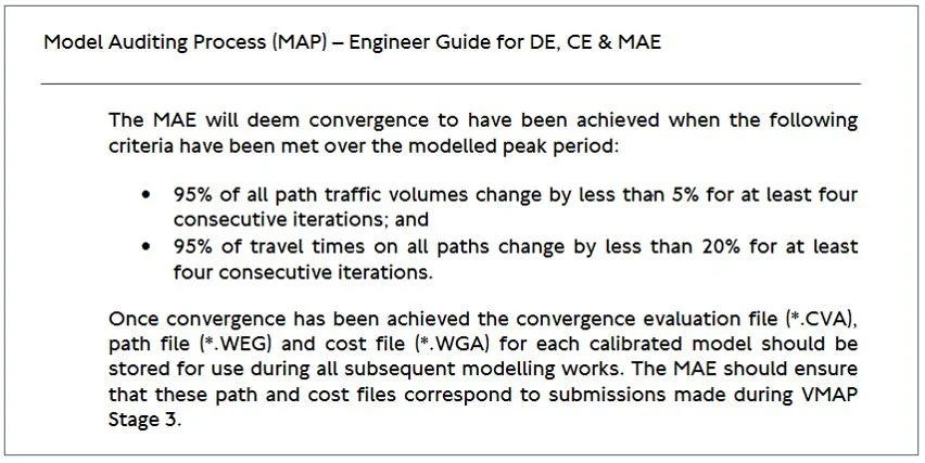
Figure 1 – TfL Convergence Criteria
TAG Unit 3.1 also contains a number of convergence indicators to check model stability, however these tend to be more suited to strategic models, rather than microsimulation models. Nevertheless, para. 3.4.5 includes an indicator which is described as “the percentage of links on which flows or costs change by less than a fixed percentage (recommended as 1%, see Table 4) between successive iterations, sometimes known as 'P' or ‘P2’ respectively.”
Our interpretation of this for microsimulation models is to output and compare the ‘Total Travel Time’ from the Overall Network Performance evaluation. This is checked for each convergence run and if the difference in Total Travel Times is within 1% for four or more consecutive iterations, then the model is considered stable.
Internal VISSIM Convergence
Within VISSIM, you have the ability to set the convergence criteria in the dynamic assignment module and then run your models until convergence is achieved.
To do this, there are a couple of tabs in the dynamic assignment module that need to be correctly configured.
Firstly, in the files tab, you need to ensure that ‘Store costs’ is ticked so that the costs for each run can be stored and assessed (see Figure 2).
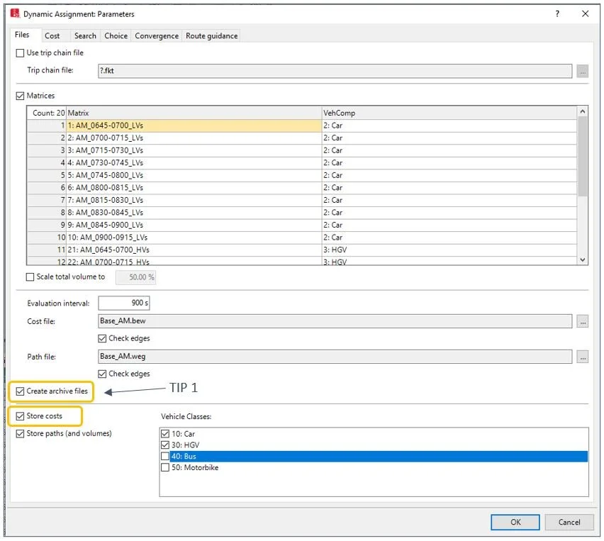
Figure 2 – Dynamic Assignment - Files
TIP 1: It’s a good idea to tick the ‘Create archive files’ so that the cost (*bew) and path (*weg) files are saved for each run. This is really helpful when you are assessing the level of convergence for each run, as you have each of the saved *bew and *weg files to choose from.
Secondly, you need to set which convergence criteria you want to run. This is done in the Convergence tab, as shown in Figure 3.
TIP 2: There are a few options available for the behaviour upon convergence:
1) You can set it to stop, and the model batch run will end once the selected convergence criteria is achieved.
2) Alternatively, you can set it to ask, and you will then get a pop up box asking if you want to continue running the simulation for more runs once the selected convergence criteria is achieved.
3) Finally, you can set it to complete all runs, and the model will complete the batch runs based on the number s you’ve chosen in the ‘simulation – parameters’ menu.
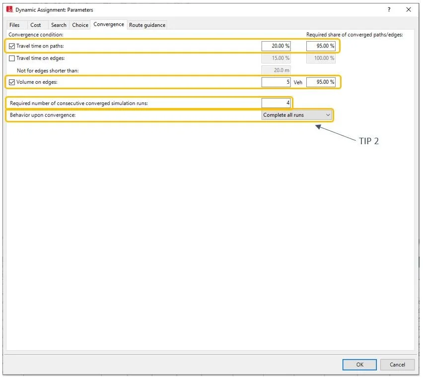
Figure 3 – Dynamic Assignment - Convergence
Once you’ve set up your dynamic assignment appropriately, the only other thing to remember is to update your ‘evaluation configuration’ to collect the convergence (*cva) files. This can be found in the Direct Output tab, as shown in Figure 4.
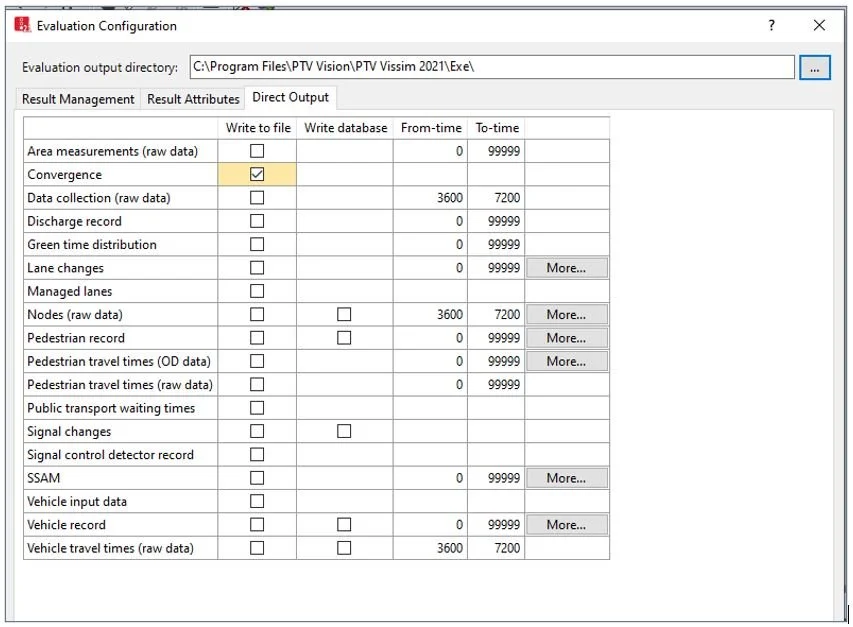
Figure 4 – Evaluation Configuration – Convergence Outputs
Having run your models for convergence, you then need to assess the outputs. This can take various forms, but as an example, Figure 5 shows how we analyse the outputs from the *cva files.
It should be noted that the above analysis was based on running the model through for the full 10 runs and not stopping once convergence was achieved. This allowed the results from all runs to be analysed and presented. For this particular project, the *bew and *weg files associated with Run 9 were used as this had 100% of the paths and edges meeting the TAG/TfL criteria, as well as having four consecutive prior runs with the Total Travel Time of 0% difference.
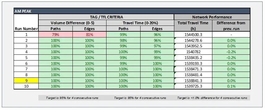
Figure 5 – Example of Convergence Analysis using *CVA files & Network Performance
External Convergence Check – Path Files
Whilst using the internal VISSIM convergence check is a useful indicator of model stability, there is one important point to note.
PTV’s Frequently Asked Questions link for VISSIM (https://www.ptvgroup.com/en/solutions/products/ptv-vissim/knowledge-base/faq/) includes some commentary on Convergence under the Dynamic Assignment option. Article #VIS29422 (https://www.ptvgroup.com/en/solutions/products/ptv-vissim/knowledge-base/faq/visfaq/show/VIS29422/) states that:
“Note: A path is converged if the convergence criterion is met in all time intervals. From the *.cva file, you cannot recognize if the paths that converged in one time interval are the same that converged in another. However, you can open the Paths list in PTV Vissim (Traffic > Dynamic Assignment > Paths), and if you add the attribute Converged (Conv) to this list, then you can see if the path is converged or not.”
The sentence highlighted in yellow is the key bit, whereby the *cva file only shows the paths/edges that fall within the convergence criteria, but these could be different from one time interval to the next.
As alluded to in PTV’s article, the use of the Paths list is something that can be used to undertake more detailed checks of the convergence levels and in particular, identify if a specific path has converged across all of the time intervals.
To make best use of the Paths list, there are two things to consider:
1) Make sure that you have ‘autosave after simulation’ highlighted so that you create a paths *att file after each simulation run.
2) Set up your Paths list to include the appropriate attributes to be recorded. As an example, our set up of the paths list is shown in Figure 7.
The reasoning behind our choice of attributes is that they form a number of checks that we undertake to determine if the paths are converged. A brief description of each of the checks is as follows:
The use of ‘Converged’ allows a very quick check to be made on which of the paths converge against travel times.
The use of ‘is detour’ allows us to filter out paths which are not required to be analysed as they are considered a detour. This is based on the path pre-selection parameters within the dynamic assignment module.
The use of ‘Path travel times (new), (old) and (raw data)’ allow us to check if a path is within a 20% difference for all of the time periods and between the different seed runs. ‘Vol (new)’ is also used to calculate the Share of Converged Path Travel Times (similar to the output in a *cva file).
The use of ‘Volume (new) and (old)’ allows us to check if the volume difference is within 5 vehicles for all of the time periods and between the different seed runs.
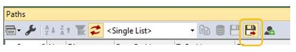
Figure 6 – Paths – Ensure Autosave is Active
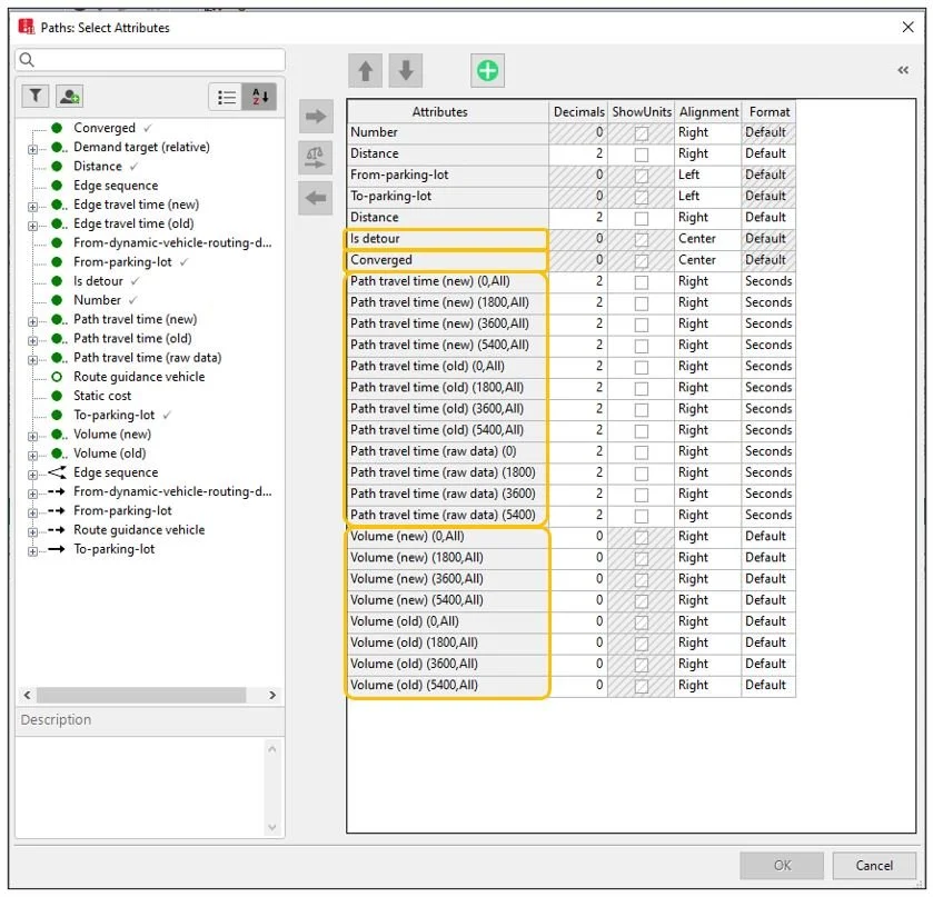
Figure 7 – Paths – Select Attributes Configuration
As with the internal VISSIM method, you then need to analyse the outputs once you have run your model through for convergence. This can take many different forms, but to show you an example of how we analyse using the Path files list and Network Performance, see Figure 8.
Other Convergence Options
There is a chance that a model could be too complex or too congested to achieve convergence against the criteria chosen. If this is the case, we recommend reviewing PTV’s FAQ link (https://www.ptvgroup.com/en/solutions/products/ptv-vissim/knowledge-base/faq/visfaq/show/VIS29421/) which offers guidance and tips on what to do if a model is struggling to converge.
Our advice, based on PTV’s guidance, would be to consider the following:
Reducing the traffic volume in congested networks is a sensible option (and something recommend by TfL in their guidelines), but make sure the percentage you choose is still suitable enough to provide a realistic network operation.
Using long evaluation intervals is a good option and you should make sure that this is higher than the largest travel time in the network, so that complete journeys can be considered in each evaluation interval.
Spend some time setting up the path pre-selection parameters for your model. Reduce the number of paths to a sensible number and make sure that the ‘avoid long detours’ factor is an appropriate value. If you also ensure that ‘correction of overlapping paths’ is ticked in the path choice model, then this should remove any unrealistic routes.
If you find that you are still struggling to achieve convergence even with all these adjustments and a significant number of runs, then it may be that your model is as stable as it’s going to be. If this is the case, it’s worth checking with any external auditors to understand if they would be happy accepting a model that’s not quite fully converged, but that has more random seed runs for results to compensate.
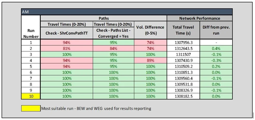
Figure 8 – Example of Convergence Analysis using Path files & Network Performance
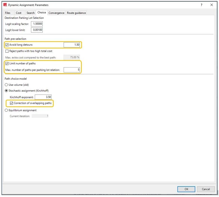
Figure 9 – Path Pre-Selection Parameters
Summary
We hope this post has helped to provide a bit of insight into model convergence and a couple of methods available if you complex and congested models that use dynamic assignment. Hopefully, there are some elements you can take away and apply to your own models.
Thanks for reading!